A Smarter Way to Use the Strengths of Your Instrumental Variables

In this post, Nick Huntington-Klein explains how you can exploit variation in the effects of instrumental variables in different subsamples to improve the performance of your IV estimations.

Instrumental Variables

The process of trying to identify causal effects from observational data is a complex one, which requires thinking carefully about where the data came from, how the world works, and what kind of barriers might lie between correlation and causation. Despite all the differences in context and theory, many causal research designs end up being implemented using one of a relatively small set of tools. One of those tools is instrumental variables estimation. I’ll be talking about my recent Journal of Causal Inference publication and how it improves instrumental variables estimation, but first let’s cover what that is, exactly.

When you’re trying to estimate the effect of some treatment D on some outcome Y, an instrumental variable is something that acts as a source of randomization for D. To take a classic example from Joshua Angrist, if you want to know the effect of serving in the military (D) on your earnings later on (Y), you can’t just look at correlation – obviously, plenty of things are related to both choosing to enroll in the military and your later earnings. The correlation includes the causal effect you want, but also lots of “other stuff” that it’s hard to see through.

And you also can’t get the effect by running an experiment – nobody’s going to let a researcher come in and randomly assign people to join the military. But maybe the world already ran an experiment for us! In the Angrist paper, he looks at the Vietnam draft, where the order in which you were drafted (and thus your chances of ever being called up) were based on a random ordering of your birthdate. Like an experiment! Unlike an experiment, though, people are also choosing on their own whether to enlist without being drafted, or evade the draft.

The solution is to use your birthdate as an instrumental variable for enlisting. Use your birthdate to predict how likely you are to enlist in the military. This prediction isolates only the random part of enlistment, not the “other stuff” part. Then, use your enlistment predictions in place of actual enlistment. You’ve isolated just the part of the correlation between D and Y that reflects the D → Y relationship. Awesome.

There’s Always a “But”

Instrumental variables aren’t magic, though. We need to be sure that they’re really as experiment-like and random as possible while still somehow being related to treatment. That’s the validity assumption, and it’s a whole long thing and researchers love to quibble about it, I won’t go into it here.

However, there are also some statistical weaknesses with instrumental variables. Instruments have to be relevant, meaning that they aren’t just related to treatment but strongly related to treatment. If the draft assignment only made a few people enlist in the military, then the prediction will be weak and there won’t be much we can do with it! Estimates of causal effects get very noisy. The problem gets much worse in small samples.

Instruments also need to have monotonic effects. That is, they need to affect everyone in the same direction. If most people are more likely to enlist in the military if drafted, but there are a few people out there who somehow become less likely (perhaps they were interested in enlisting until someone told them they had to, and now are going to draft-dodge), then it messes up the whole procedure. These people get included in estimation, but backwards because of their opposite effect, and so the more positive the effect of enlisting would be for them, the less positive our estimate will be. Oops.

Improving Relevance and Monotonicity

That brings us to the paper “Instruments with Heterogeneous Effects” in the Journal of Causal Inference. This paper looks seriously at the issue that the instrument may have really strong effects on your propensity to be treated for some people but weak effects for others. Maybe some positives and some negatives, but also maybe just some positives and some even-more positives and some nearly-zero-but-still-positives.

A big problem here is that traditional instrumental variable estimation methods take everyone’s effect and pools it all together. So if you have a bunch of people in your data who don’t care about the instrument, they add basically nothing to your estimate but drag your relevance down! Freeloaders!

The fix is pretty obvious: don’t pool everyone’s effect together! We can follow some basic steps (which are automated in the R and Stata packages linked in the paper):

1. Use some method that lets you estimate the effect of the instrument differently for each person. There are plenty of “heterogeneous treatment effect” methods springing up these days in machine learning, like causal forests, that can be used for this.

2. Split up the sample by how effective the instrument is for them – strong effects in one group, middling effects in another, weak effects in another, opposing-direction effects in yet another (or some number of splits other than four).

3. When using the instrument to predict treatment, allow each of these groups to have their own effect.

That’s about it! This process lets those weak-effect freeloaders see themselves gracefully out. It lets the people for whom the instrument is predictive (who we were thinking about anyway when we came up with the research design) to run the show. And even better, it helps with our problem with monotonic effects. We don’t actually need the whole sample to have an effect in the same direction – as long as everyone is in the same direction within each of these groups we’re good to go! So if we can figure out who these opposite-sign effect people are in Step 1, that problem is solved.

So Does it Work?

This procedure, despite requiring very little effort on the part of the researcher, no super fancy tools, and working in pretty much any scenario, helps strengthen our estimates by quite a bit!

I test the method using another Angrist paper, this one with Battistin and Vuri on the effect of small class sizes. What’s a source of random variation in class sizes? They look at Italy, where there are maximum class size limits of 40 students. If you’re in a school that happens to have 39 kids in your grade, you’re probably in a classroom of 39 students. But if you’re in a school that happens to have 41 kids in your grade, they have to split you up and you’re going to be in a much smaller 20 or 21-person room. Whether your grade happens to have 39 or 41 students that year seems pretty random! And so it serves as an instrument.

They have a pretty big sample size and an instrument that would by conventional measures be considered not to have a problem with relevance. So I take subsamples of that data and see how close I can get to that full-sample estimate. If, using a small sample, I can get much closer to the full-sample result than traditional instrumental variables, that tells us that I’ve tamed the relevance problem at least a bit, and we don’t have to worry as much about sampling variation. Results are in Figure 1.

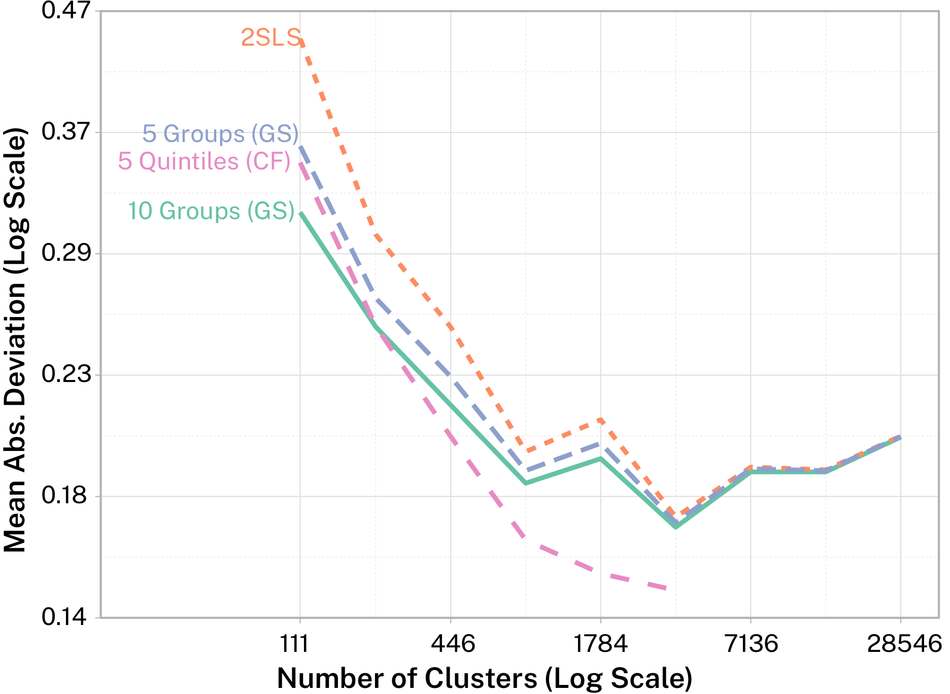
In the figure, lower values means less sampling error – it’s like prediction error except we’re “predicting” an effect rather than an outcome. 2SLS is a traditional method, and the other three represent different ways of doing what I’m talking about, with different approaches to estimating the different groups.

In small samples, the traditional method is definitely trumped. Even the “GS” methods work – these are entirely brainless ways of splitting the sample into groups that simply entail guessing at some group divisions a few times and seeing what sorta works. As the sample size gets bigger, the relevance problem lessens for the traditional method and the GS methods aren’t much of an improvement.

But the CF method – using causal forests from machine learning to do the splitting – continues to work well! We’re doing a much better job at pulling the true effect out even in relatively large samples.

Conclusion

Instrumental variables are an important tool to have in your back pocket. There are plenty of real-world situations where we can think of some random-like mechanism that assigns treatment for us. Heck, I’ll take an “experiment” where I can find one. But finding the right setting isn’t enough. We also want our estimation to get as much out of the data as we can. I provide one very simple improvement on the traditional method that goes looking for the observations that are most helpful, getting us as close to the right answer as possible even with less data at our disposal.

Tags

Share