Bootstrap Your Way to Better Experiments

In this post, Simon Grest, Data Science Lead at the Netherlands' largest food retailer Albert Heijn, shows how using bootstrapping with historical data can be used to validate different estimators in A/B testing.

On randomization

Randomisation of treatment and control groups is the go-to approach to making robust statistical inferences about causality. In experiments with interventions in the physical world, practical considerations often constrain how randomisation can be done, possibly leading to biased results or reducing the sensitivity of the experiments.

When experimenting in the context of time-series data it is possible to use stronger assumptions to mitigate these limitations and improve the sensitivity of experiments without biasing the results.

This piece compares standard A/B testing with two different estimators of treatment effect and shows how using bootstrapping with historical data can be used to validate these estimators.

In-store experimentation and the limitations of A/B testing

Experiments run on Albert Heijn’s website ah.nl usually fit the classical framework of A/B testing well, but running experiments within stores is usually more complex.

Unlike on the website it is often not desirable or even possible to allocate a different treatment to different customers who enter a store. It’s not possible to change the position of products on shelves only for some customers and not others for example. Furthermore experiments in stores are usually more expensive (and risky) to run and therefore scaling of experiments is limited.

As a result experimenting in stores often means choosing a relatively small subset of stores to receive the treatment. This choice can be made at random in order to eliminate any biases that might come from differences between stores. The limitation on the number of stores in the trial means however that the variation in measurements will be high and a comparison between the treated and control stores in the style of an A/B test will not be able to distinguish smaller treatment effects from randomness.

An imaginary experiment: Brighter lighting attracts more customers

Suppose that research suggests that customers prefer brighter lighting while they are shopping. An experiment is going to be run to test the hypothesis that increasing the brightness of the lights will lead to more customers.

The costs associated with adding the required lighting mean that an intervention can be trialled in only twenty out of the approximately one thousand stores of Albert Heijn. These twenty stores can be selected at random, and the remaining stores will continue with normal lighting and can therefore be seen as a control group. The intention is to run the experiment for a four week period and then analyse if the change in lighting has led to any change in the number of customers that came into the experimental stores.

Estimating treatment effects

How can the effect of the lighting on the number of customers in the stores in the trial be estimated? In addition to A/B testing the below section briefly introduces two possible alternative estimators of treatment effects that can be used with time-series data.

For the purposes of illustration an extra 100 customers per week per store were added to the actual measured number of customers for the treatment stores during a simulated four-week intervention period.

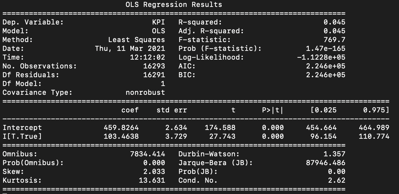
A/B testing

The typical approach for an A/B test in this experiment would be to compare the average customer count per week in the treatment group with the average customer count per week of the control group during the treatment period. The treatment effect is then estimated as the difference between these two averages. The variability of the number of daily customers in all stores throughout the four-week period can be used to compute confidence intervals for the estimate of the treatment effect.

A neat way to compute this estimate is to use a simple linear regression for the number of customers during the treatment period.

NCₛₜ = α + β×Iₛ + 𝛆

where NCₛₜ is the number of customers for store s at time t and Iₛ is 1 for treatment stores and 0 for control stores. α is the intercept term and 𝛆 represents the error term or alternatively effects that come from sources outside of those in the model. The resulting value of the coefficient β can then be interpreted as the number of customers added due to the change in lighting per week per store.

The python statsmodels.formula.api module can be used to achieve this:

model = smf.ols(formula = "NC ~ I", data = df).fit()

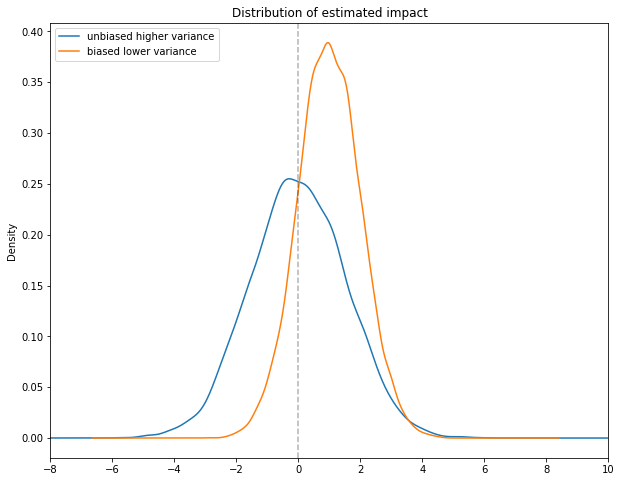
Running model.summary() the estimated daily impact of 103.4638 units can be found in the result table:

Difference in differences (DiD)

The difference in differences estimator uses the average number of customers for the treatment and control groups in both the pre-intervention and post-intervention period. The difference between the control and the treatment group are calculated in both periods and the treatment effect is estimated as the difference between these two differences. The below animation from the Harvard / Stanford collaboration the Health Policy Data Science Lab illustrates the idea nicely:

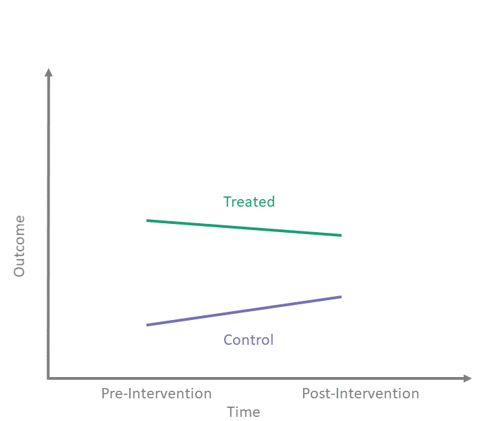
The core assumption that the DiD estimator makes is referred to as the parallel trend assumption — the idea is that in the absence of the treatment the number of customers in the control and treatment groups would have moved in parallel through time.

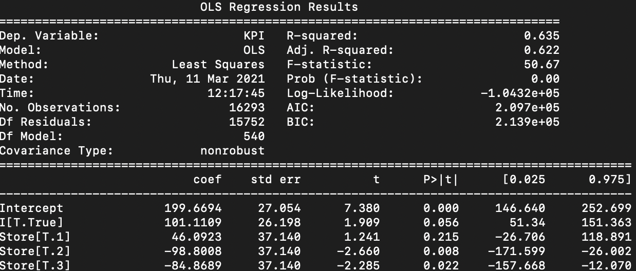
Practically this estimator can also be calculated using the regression equation:

NCₛₜ = α + β₀×Iₛₜ + Σɣₛ×Jₛ + 𝛆

In this case an indicator variable that is dependent on time and the store is used — Iₛₜ takes the value 1 where the store is in the treatment group and the week is in the intervention period, otherwise it is 0.

Additionally to allow for different baseline levels of customers in different stores, the coefficients ɣₛ are introduced — this is equivalent to allowing each store to have it’s own intercept variable. The indicator variables Jₛ take the value 1 for store s and 0 otherwise.

In this case the estimate of the treatment effect is the fitted value of β₀ or in the python output the value of 101.1109.

Causal Impact

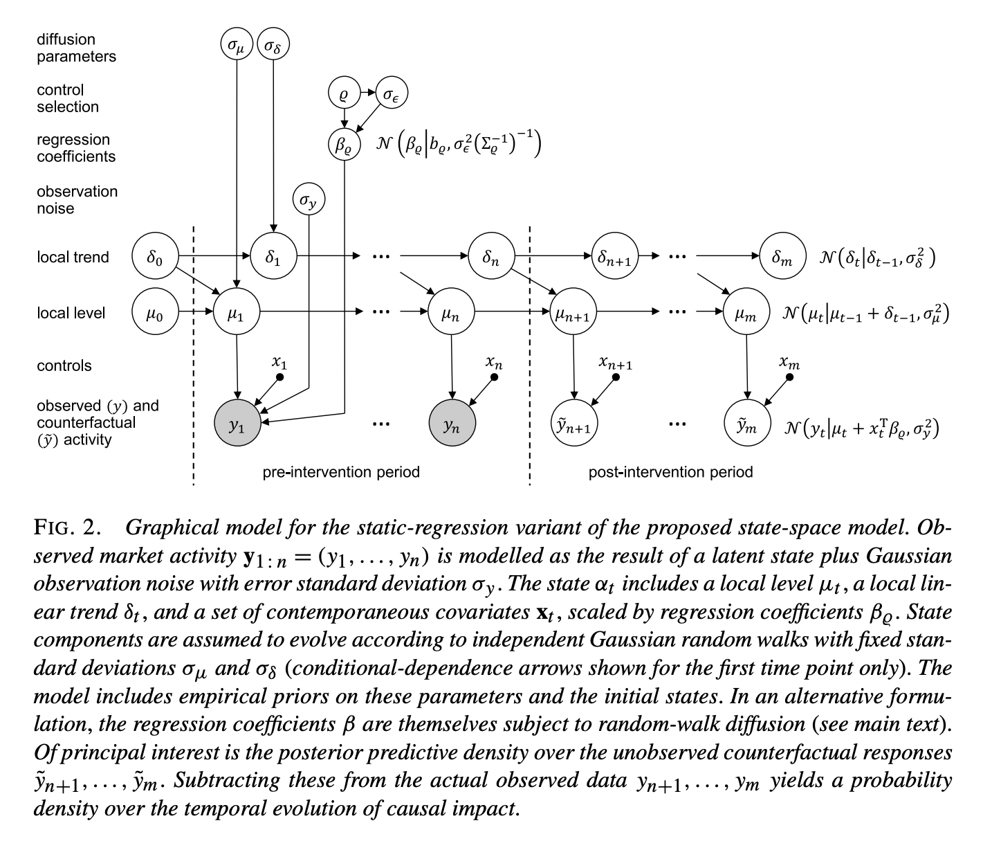
The final estimator used is based on work published by Google research in 2015. The idea behind the causal impact approach is to fit a model on the historical pre-intervention relationship between the number of customers visiting the control stores and the number of customers visiting treatment stores.

This fitted model can then be used to estimate a counterfactual for the number of customers visiting treatment stores in the intervention period. In other words, given the number of customers visiting the control stores in the intervention period how many customers would be expected in the treatment stores if there had been no change in lighting. Under the hood, the Causal Impact library uses a more complex Bayesian state-space model but also makes a form of parallel trends assumption.

Google Research provides an R implementation for Causal Impact. For illustration the CausalImpact model estimates the average number of customers visiting stores in the treatment group by using the average number of customers visiting the stores in the control group. More info about how to use the library can be found on the Google Research Causal Impact page.

A visual and numerical summary is produced by the R implementation of the Causal Impact model. The visual summary shows three panels all of which display twelve weeks of the pre-intervention period and then the four weeks of the intervention period. The grey vertical dashed line divides time between the pre-intervention and post-intervention period:

• The first panel uses a solid line to show the average number of customers visiting treatment stores per week while the dashed line shows the predicted average number of customers based on the actual number of customers observed in the control stores — this estimate is the counterfactual — how many customers would there have been if there was no change in lighting.
• The second panel shows the difference between the counterfactual estimate and the actual measurement.
• The final panel shows the cumulative impact of the difference from the second panel.

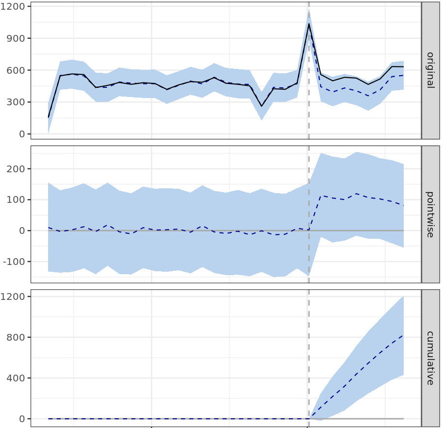
The estimated treatment effect per week per store or Average AbsEffect can be read from the top right corner of the table as 102.9132.

Bias and variance of estimators

All these estimators appear to have approximately correctly picked up the 100 customers per store per week increase that was introduced into the data, but how is it possible to be confident that they will work with real intervention data?

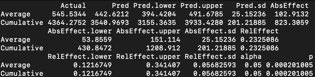
In order to understand the statistical properties of an estimator, a series of simulations of the experiment can be run based on historical data, and for each simulation an estimate can be calculated. The resulting distribution of estimates can be used to reason about the estimator’s behaviour. Drawing at random repeatedly from data in order to make statistical conclusions about the data is known as bootstrapping. Ideally the distribution of the estimator should be unbiased — i.e. centered around the true effect, and the distribution of the estimate should vary as little as possible — i.e. it should have minimal standard deviation.

A/A testing

Simulating possible effects from interventions is complicated because it requires making assumptions about what form the effects take. Would the number of customers added due to lighting changes be a proportion of the existing customers, or would they just be a constant, would the effect be larger at weekends, how much would the effect vary across different stores?

In contrast in the historical data there is only the regular lighting, i.e. no treatment, and there is consequently no effect. If the effect is measured on historical data the expected effect should be zero. By repeatedly drawing random subsets of twenty stores from the data and estimating the effect size relative to the remaining stores, a statistical picture of the distribution of the estimator can be established. Testing an estimator in this manner is sometimes referred to as A/A or placebo testing.

Bootstrapped A/A simulation results

A/A tests were simulated for the three different estimators (A/B testing, DiD and CausalImpact) by drawing samples of 20 stores 10,000 times and then estimating the treatment effect with each of the estimators.

A/B testing vs DiD

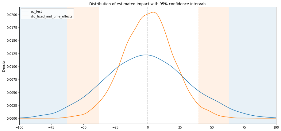
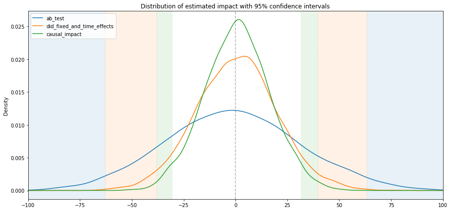
Comparing the distributions of estimations for the A/B testing and the DiD estimators, it can be seen that both estimators appear to be unbiased (centered around zero), but that the variability of the DiD estimator was significantly lower than that of the A/B testing estimator.

Practically the difference in variability means that the DiD estimator is more sensitive (or powerful). If a 95% confidence interval is considered, then treatment effects with a magnitude between 40 and 60 customers per week will be statistically significant for the DiD estimator but not for the A/B testing estimator — this corresponds to the orange vertical bands in the below figure. Therefore treatment effects with a magnitude between 40 and 60 can be detected by DiD but not by A/B testing.

A/B testing vs DiD vs Causal Impact

Adding the CausalImpact simulation to the above analysis, it can be seen that it is also unbiased, and that the variance is lower still than that of the DiD estimator. Effects with a magnitude between 30 and 40 can be detected by CausalImpact but not by the DiD estimator — this area is coloured in green in the below figure.

Conclusion

In this simulation CausalImpact proved to be better than both the DiD and the A/B testing estimators — all three gave unbiased estimates of the null treatment effect but CausalImpact had lower variance than the other two estimators and was therefore capable of detecting smaller effects.

In the imaginary example of the experiment with store lighting, simulations showed that the standard estimator associated with the A/B testing approach would fail to detect an average change of less than 60 customers per week over the four weeks, while CausalImpact was sensitive enough to detect an change in the average as small as 30. It is important to remember that this extra statistical power has been gained by making strong assumptions. If these assumptions are violated, for example if the parallel trends assumption is broken or if there is a break in the historical relationship between the control and treatment stores, the estimators result may become biased, and the confidence intervals unreliable.

Ultimately the simple difference of means associated with A/B testing remains the most robust of the three estimators, but at the cost of being able to detect smaller effects.

This post was originally published by AH Technology on Medium.

Tags

Share