How to Use Previous Model Deployments to Build (a Better) Causal Model

Do you experiment with different models in production? Sam Weiss from Ibotta on how you can use observational causal inference to build a better model on data from previous model deployments.

Introduction

Causal Uplift (or heterogeneous treatment effects) models estimate the treatment effect at an individual basis and have been found to be more performant in practice than predictive models. I have written about evaluating, developing tradeoffs and building them before using experimental data. However, it’s often prohibitively expensive to run randomized experiments to gather data required to build uplift models. Practitioners often turn to observational causal inference methods in order to estimate these models. In practice, these methods often offer sub par performance relative to building off of random experiments because the assumptions required of these methods do not hold.

In this post, I will discuss how one can use previous rules based model deployments to estimate the underlying causal effects of treatments. Under conditions described below, one can be sure that the assumptions of observational causal inference hold. With this data, one can build an uplift model without running new randomized experiments.

First I will describe why randomly assigning treatments is preferred. Then I will go into the necessary assumptions when the treatments are not randomly assigned and why those often do not work in practice. I will then describe how previous model experiments can be used to determine the causal effect of the underlying treatments. Finally, an example using <code>mr_uplift</code> is shown.

Experiments as The Gold Standard

As has been said ad nauseam, “association does not equal causation”. A common reason being is that there could be other variables that effect who received the treatment or not.

The most effective way of estimating a causal effect is therefore to run an experiment and randomly assign the treatments. This ensures that there are no other differences in treatment groups other than the effect of interest. In this case, the measured association is equal (in expectation) to the causal effect. However, in many cases we cannot run a random experiment due to either costs or ethical considerations. For these, we have to rely on data we observe in the ‘wild’. As stated above, the biggest issue with measuring associations with this kind of data is that there are almost always other variables that effect which individuals receive which treatments.

This means that the association effect you’ll be calculating is the sum of the treatment effect along with all other differences between the treatment groups (see Angrist and Pischke p.11). And since those differences are almost always larger than the treatment effect you’re trying to estimate, simply measuring the association between the treatment and response will result in a biased estimate.

Observational Studies

Observational causal methods attempt to control for these differences in who received the treatment. In essence, they try to make the two treatment groups as similar as possible so that the only difference between them is the treatment. There are numerous ways to do this, but some of the more common are to use propensity models to either weight observations or match them. There are lots of great tutorials out there that describe these assumptions and how they work in practice to create propensity scores. A few you can find here, here, and here.

These methods rely on two assumptions. At a high level, they are:

• Ignorability: You controlled for all the relevant variables that cause differences in which individuals received which treatments.
• Support: There there is non-zero probability that an individual received the treatment in the data.

Ultimately, an observational causal study’s success or failure is determined by whether these assumptions are true. Unfortunately, they are often not. For example, there could be a variable that causes whether an individual is in the treatment group, but you don’t observe it. In this case, the ignorability assumption is violated. A great paper that discusses these methods in practice and results can be found here.

Since naively controlling for variables often leads to poor results, researchers often rely on domain knowledge to identify the causal effects more accurately. Specifically, they try to find cases where a treatment is (arguably) randomly assigned in the ‘wild’ and use that to measure the treatment effect. In the rest of this post, I describe such a case I’ve seen in practice that can allow a data scientist to measure the treatment effect using previous deployments of models. I believe the conditions described here are common enough that others might find it useful.

Experimenting with Rules Based Models

As stated above, experimenting with underlying treatments is often an expensive task. In practice, I’ve seen businesses and data scientists experiment with the different rules that assign treatments instead. I believe this is a more common setup than experimenting with the underlying treatments because it’s easier to get ‘buy-in’ from stakeholders and is cheaper.

Here, I’m defining “Rules Based Model” as a deterministic function that maps an individual’s variables to a decision. There can be many different ways to go about doing this; one might use a variable of an individual’s history to split or a probability measure from a machine learning model.

For example; in a subscription based business, a marketer might give a costly monetary reward to users most likely to churn in order for them to renew. In this case, you might have the probability of churn for all users, and assign the reward to only those that have a high probability of churning. At Ibotta we’ve deployed these kinds of rules based models often. Of key interest to this analysis is that we experiment among different kinds of rules. In this churn example, we might have multiple different rules based off the same probability measure but with different cutoffs. For instance; one rule might say that we assign the reward to users with greater than 50% probability of churning, while another uses anything greater than 75%.

In this scenario, a data scientist can use this information to measure the causal effects of the underlying treatments for some users. The ignorability assumption is valid because we have access to the relevant variables used to assign the treatment (the probability of churn). However, the support assumption is dependent on the user and models used and will potentially restrict the treatments we can measure for different users. Below, I argue that this kind of setup can be used to accurately estimate the underlying treatment effects.

Example Rules Based Model Experiment

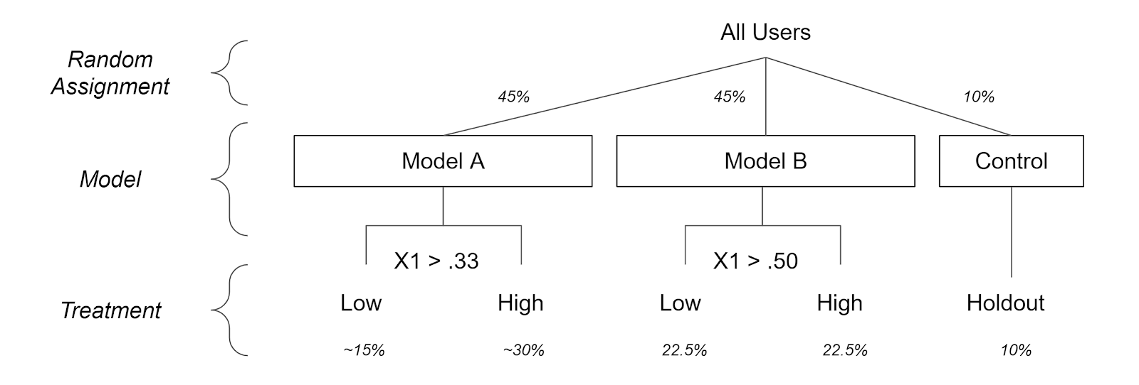
In this scenario, I am assuming there are two ranked treatments: a high one and low one. There is a particular variable X1 that different models split on. Those users that have a higher X1 value are believed to respond stronger to the high treatment. Because of this assumption, those that have higher values of X1 are assigned the higher treatment. However, there is uncertainty as to what that cutoff point should be that designates users between a high and low treatment. Therefore, there is an experiment between two models and a control to determine the cutoff.

While Model A assigns those with values of X1 above .33 the high treatment Model B uses .5 to assign the high treatment. The percent of users in Model A, Model B and the Control is 45%, 45%, and 10% respectively. Below is a graph of the setup. (X1 is assumed to be uniformly distributed without loss of generalization). Below is the assignment process for users.

Since the models and control were randomly assigned we could look at the averages of user behavior in each model or control group. This will answer the question ‘what will happen if we give a user one of the different models?’ That’s great to determine such metrics like the ROI of a model or which model provides more user activity.

Instead, uplift models want to ask a different question ‘what will happen if we give a user one of the different treatments?’ Since the treatments themselves were not randomly assigned, we will have to take into account the data generating process using X1. To better see this, let’s take another look at how the models were assigned based of the X1 value below:

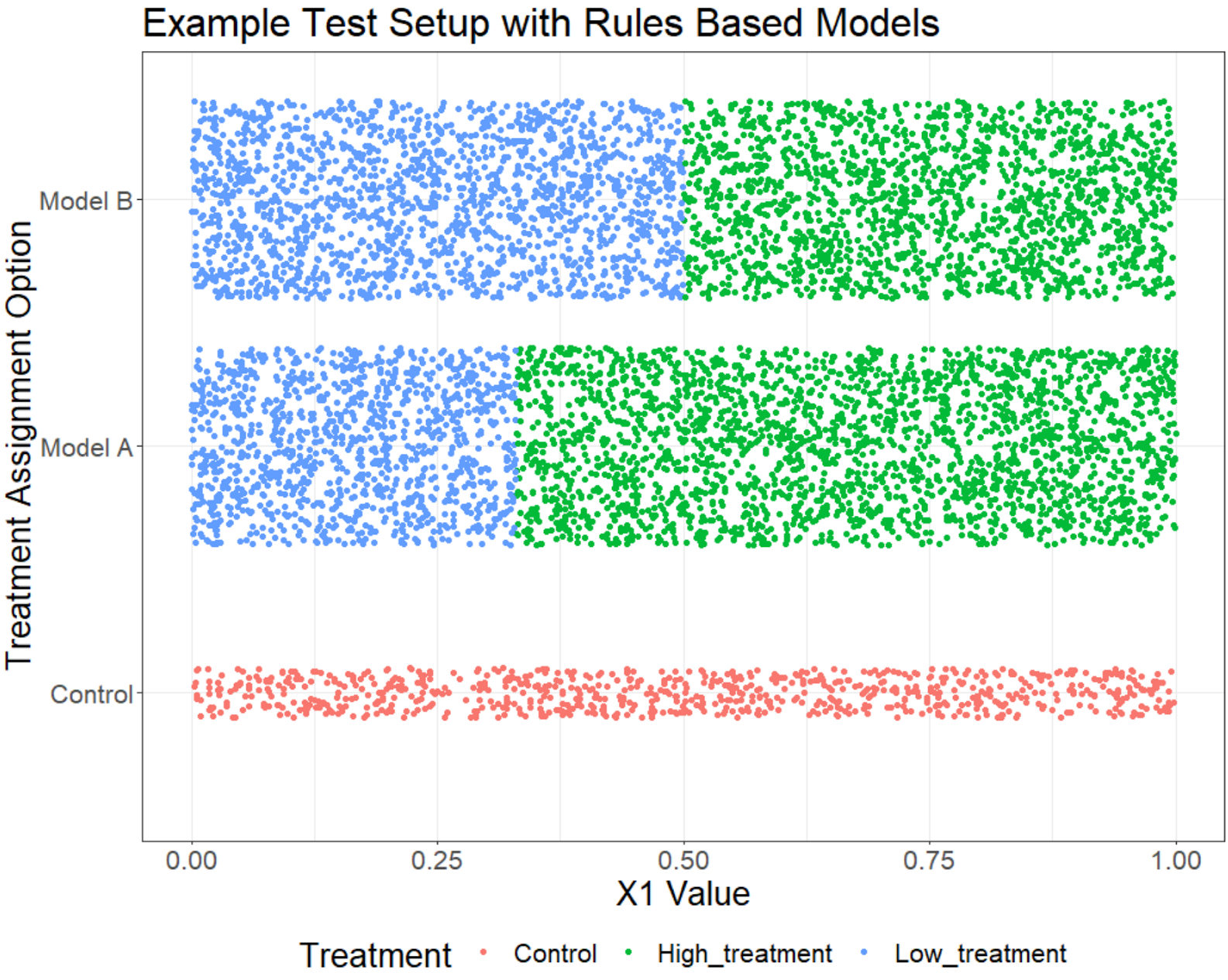
Above each point is an individual. On the x-axis we see the values of X1 and on the y-axis we see the model assignment and each color is the treatment assignment.

We can see that different values of X1 lead to different distributions in the realized treatment groups. For instance, those that have X1 less than .33 have a ~78% probability to receive the low treatment and a ~22% probability of the control. We can therefore use propensity weighting to estimate the causal effect of either the low treatment or the control for this group. To further see which groups of users have support over treatments, I break them out into each ‘Support Groups’ below.

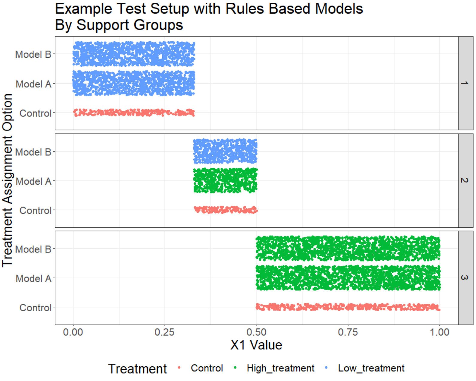
In this example, there are three distinct support groups that have different treatment distributions. In this scenario they are functions of one variable, but in general can be an arbitrary number of variables — the important thing to remember is that we have access to all the necessary information. Those that have values below X1 (group 1) are assigned either the Low treatment or control, while those that have values of X1 above .5 (group 3) are assigned the high treatment or control. Those in between (group 2) have support over all treatments.

Without further assumptions, we cannot calculate the causal effect of the high treatment on group 1 individuals because no one received a high treatment in that group. Similarly, we cannot estimate the causal effect of the low treatment on users in group 3.

Here we can see that for certain users we can estimate the causal effect for some of the treatments. The two assumptions are valid because:

• Ignorability: We have access to the underlying data (X1 in this case)used in assigning these models. We know no other variable causes the treatment assignment.
• Support: Here we will have to restrict our measurement of treatments to those subgroups of users that have received them. We can estimate which users have low probabilities of receiving a treatment and exclude those treatments on a user level basis.

In mr_uplift

As I’ve discussed previously, the <code>mr_uplift</code> package estimates the uplift (or heterogeneous treatment) effects of several treatments on multiple responses. It measures the trade offs among competing objectives (e.g. costs vs growth) a business might have in deploying these models in often ambiguous environments. I have updated the mr_uplift package to include functionality to estimate these kinds of experiments using propensity score weighting. Here is a notebook for a more in depth explanation.

Briefly, it builds a random forest to calculate the probability of a treatment given the explanatory variables. It then uses the inverse of those estimated probabilities to weight individual observations in the model building process. Weighting this way will estimate the causal effect of different treatments accurately given the assumptions of observational causal learning.

However, not all individuals have support for all treatments. There is an option of propensity_score_cutoff that specifies when a treatment could be assigned to a user. This is the inverse of the probability a user receives a treatment. The default is 100 which corresponds to a 1% probability that the individual is assigned a treatment. Anything higher than that will not be used for that individual in either the model building or prediction steps. Below is an example of using propensity score functionality within the mr_uplift package. I assume there is a single response variable y, explanatory and treatment assignment variables x, and treatment variable(s) t:

from mr_uplift.mr_uplift import MRUplift
uplift_model = MRUplift()

param_grid = dict(num_nodes=[8, 64], 
             dropout=[.1, .5], 
             activation=['relu'], 
             num_layers=[1], 
             epochs=[25],
             batch_size=[512], 
             alpha = [.99,.9,.5,.0], 
             copy_several_times = [1])
uplift_model.fit(x, y, t, param_grid = param_grid, 
                 n_jobs = 1, use_propensity = True, pca_x = True, 
                 optimized_loss = True, 
                 propensity_score_cutoff = 100)

Here I’ve applied some preprocessing using the option pca_x and use a loss function specifically designed to measure the heterogeneous treatment effects with the option optimized_loss = True (see here). By default, mr_uplift will automatically subset to treatments that have high support for each user and then calculate the optimal treatment. This ensures that the support assumptions holds.

uplift_model.predict_optimal_treatments(x_new)

However, the data scientist is free to explore all treatments for all users by setting use_propensity_score_cutoff=False. There’s no guarantee the model will be able to extrapolate correctly to treatments where specific groups of users haven’t been exposed to them, but the option is there to explore. Finally, all other aspects of mr_uplift remain the same and you can use this functionality to estimate tradeoffs as before.

Example at Ibotta

At Ibotta we have a product that assigns different treatments to our users based off of their previous history of interacting with clients products. This is a fairly simple rule based model, and every deployment of this model includes a random assignment similar to the ones described above. These deployments give us a rich dataset varying over different products and time. With the new mr_uplift code that allows for propensity models, we are now able to build uplift models based off this data without running new randomly assigned experiments

One particular interesting finding was that the most important variables were not variables associated with user interactions with clients products (as the original rule based method suggested). Instead, user interactions with the app had a far higher effect. Based off these findings, we are currently revamping that product to achieve higher performance.

Conclusion

In this post, I went over traditional issues with observational causal inference. I then describe a situation where if previous experiments of models exist, we can potentially exploit this structure and learn the causal effect of the treatments for some users. If these kinds of projects and challenges sound interesting to you, Ibotta is hiring. Check out our jobs page for more information.

This post was originally published on Medium.

Tags

Share