Introduction to Dags, Their Applicability, and How They Come About

Anders Bast Olsen, master student at Copenhagen Business School, explains how actionable business insights can be derived from directed acyclic graphs and why data analytics and qualitative approaches form a powerful combination for causal learning.

Introduction

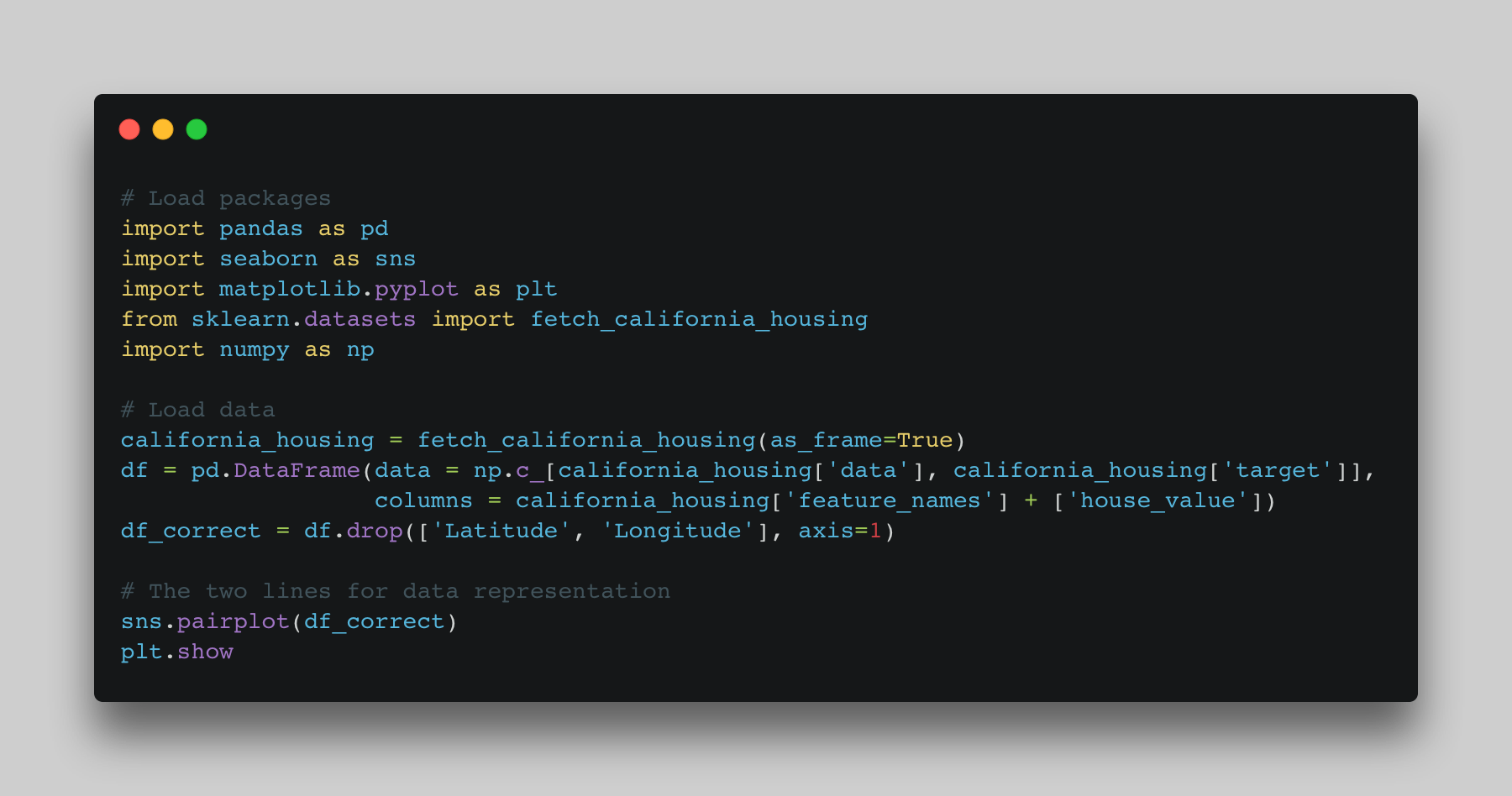
In most machine learning, the analyst’s starting point will be to get a sense of the underlying relationships in a dataset, formally known as exploratory data analysis (EDA). For EDA, a scatterplot is a popular tool to visualize the correlation between any given variables in a two-dimensional space. The popularity may in part be attributed to the ease of use, that is, with just two lines of code the underlying relationships in the data are made visible. See for instance the case of the California housing data:

# Load packages
import pandas as pd
import seaborn as sns
import matplotlib.pyplot as plt
from sklearn.datasets import fetch_california_housing
import numpy as np

# Load data
california_housing = fetch_california_housing(as_frame=True)
df = pd.DataFrame(data=np.c_[california_housing['data'], california_housing['target']],
                  columns = california_housing['feature_names'] + ['house_value'])
df_correct = df.drop(['Latitude', 'Longitude'], axis=1)

# The two lines for data representation
sns.pairplot(df.correct)
plt.show

However, such a simple tool does not necessarily lead to the best representation of the data at hand. Clearly, the best representation depends on the purpose. Let’s define one such purpose: to find the effect of x, number of bedrooms, on y, the market value of the house. Here, we are searching for a causal effect, for which an understanding of the underlying causal dependencies would be more helpful than of the correlational relationships in the data. As such, a better representation could be a directed acyclic graph (DAG), which expresses the causal relationships between each of the observed variables:

From the DAG in fig. 2, an intuitive and very useful interpretation of the causal relationships can be obtained, merely upon inspection of the arrows in the diagram. Hence, to find the effect of x on y, the DAG shows that you should control for another variable, the number of rooms. To make the life of the analyst even easier, using software packages such as causalfusion.org, answering causal effect queries can be fully automated once the DAG is known. Thus, if the analyst can formulate the query relevant for the purpose, such as,

$$ \begin{equation*} 𝑃(𝑀𝑎𝑟𝑘𝑒𝑡𝑉𝑎𝑙𝑢𝑒|𝑑𝑜(𝑁𝑢𝑚𝑏𝑒𝑟𝑂𝑓𝐵𝑒𝑑𝑟𝑜𝑜𝑚𝑠)) \end{equation*} $$

, an estimable equation for that query is returned (given it exists). In this case:

$$ \begin{equation*} \sum_{Number of Rooms}P(MarketValue│NumberOfBedrooms,NumberOfRooms)P(NumberOfRooms) \end{equation*} $$

Nothing is That Easy, Where is the Catch?

Obviously, no matter how beautiful this automated computation is, it is not magic. The computation is based on a directional and mathematical interpretation of the DAG, and several reformats of that DAG, all of which are summed up by the three rules of do-calculus. However, since these rules have already been automated and made readily available for everyone to use, the “catch” is not the underlying use of math. Rather, the “catch” is the process by which the DAG comes about. Specifically, the DAG in fig. 2 is based upon, at best, weak assumptions imposed by the author. For instance, the number of rooms has no known causes, i.e., edges pointing into it, yet it could be argued that it is partially caused by income levels in the respective area. Encoding this and other credible assumptions would lead to different DAGs than the one in fig. 2. Hence, estimating causal effects will only be valid when the DAG encodes the true underlying causal relationships in the data generating process.

From Raw Data to a Causal Model using Causal Discovery

Since the application of do-calculus, automated or not, prerequisites a valid causal model, encoding a DAG based on weak assumptions is insufficient. In fact, most of the analyst’s time is likely spent on the process of building and refining a causal model. Here, this work is referred to as causal discovery, which is then further divided into distinct approaches. Unlike do-calculus, causal discovery does not operate in a finite problem space in which completeness has been proven. As such, the discovery tends to be an iterative process, wherein methodologies range from the social sciences to math, or a combination of the two. Normally, causal discovery is defined as a fully data-driven approach wherein smart algorithms, such as the PC algorithm, are applied to a dataset to extrapolate the causal relationships found in data. Here, I will define this as the quantitative approach to causal discovery. By contrast, a more qualitative approach to causal discovery leverages methodologies from the social sciences, such as surveys, interviews, and focus groups. This involves the collaboration between domain and statistical experts, seeking to distill domain knowledge in form of DAG. Take, for example, a piece of information such as “California houses the most one-percenters in the nation since great tax reductions are offered for people building new houses.” This knowledge should then be incorporated in the DAG by including the relationship AreaIncome → HouseAge in the causal model. Most often, however, the qualitative and the quantitative approaches are combined and used iteratively.

This process is facilitated by the fact that most DAGs give rise to testable implications based on the d-separation relationships between the variables in the model. For example, in the diagram in fig. 2, the causal chain between AreaAveOccup → AreaIncome → HouseAge implies that AreaAveOccup should be independent of HouseAge, conditional on AreaIncome. This statistical relationship can be tested in the data and if found to be invalid, the DAG should be adjusted accordingly. This provides an opportunity to falsify a hypothesized causal model and thereby enables an iterative process of model-building.

Measuring Performance

After causal discovery, the performance of the uncovered DAG is inspected. In machine learning, the objective is usually to minimize some cost or error function. Critics would argue that this is actually one of the drawbacks of machine learning, as it is merely function fitting leading to no causal information. However, from a risk-management perspective, function fitting is by no means a drawback, because it enables the error rate, i.e., the difference between predictions and observable facts, to be cleanly expressed. Hence, from a machine learning model, we can, often with great confidence, say we expect the predictions to be right in n-percent of the instances and decide whether that suffices for a production-ready model. In causal inference, exactly because it is not function fitting, no such expected performance evaluation can be done. While there is generally no doubt about the performance potential of causal inference (e.g., studies show that it can replicate experimental benchmarks such as RCTs), performance is measured differently in the two realms. Clearly, when the main school of thought is built on function fitting, the inability to express performance as prediction error is a drawback that limits practical applications. Hence, to overcome this challenge, practitioners should increasingly turn their attention to performance measures based on actual business metrics rather than mere statistical measures such as goodness of fit.

Concluding Remarks

As this post demonstrated, a causal query may just as easily be answered using DAGs as it is to fit a regression-plane to a scatter plot of a set of predictors and a dependent variable (see fig. 2). However, the realm of causal inference prerequisites a causal model, which machine learning algorithms do not. To see further adoption of causal data science in practice, skills and methodological knowledge, in particular related to causal discovery, need to be diffused more widely. Yet, with the possibility of full automatization of the causal inference process based on do-calculus, and considering that observational causal inference methods are able to approximate experimental results at a fraction of the cost, it is likely that further advances will be achieved in the future. With more frequent applications and readily available tools the potential for causal learning in a business analytical context becomes tremendous.

Tags

Share